Deformable DETR a tiny Implemenation

Code

import torch 
import torch.nn as nn
print(f'torch version {torch.__version__}')

torch version 2.9.0+cpu

Overview

This blog provides a code-level walkthrough of the internals of Deformable DETR and its core component—deformable attention—to understand how it works in practice. I’ll explore the full pipeline: starting from how a batch of images flows through the convolutional backbone, then into the encoder, and finally how deformable attention operates within the architecture both in encoder side and decoder cross attention. Along the way, I’ll highlight where Deformable DETR aligns with the original DETR and where it diverges. All examples shown below are executable in the accompanying notebook and have been tested to work end-to-end.

Prerequisites

I assume the reader have good understanding of DETR

Why was Deformable DETR needed?

Deformable DETR is an enhancement of DETR, which was one of the first approaches to apply transformers to object detection. While DETR introduced a novel paradigm, it faced two major challenges

1. Difficulty Detecting Small Objects

Most modern object detection networks leverage Feature Pyramid Networks (FPN) to handle objects at multiple scales. However, DETR cannot easily incorporate FPN because its global self-attention operates over the entire feature map, making multi-scale attention computationally expensive. Deformable DETR addresses this by introducing multi-scale deformable attention, which selectively attends to a small set of key points across different feature levels instead of the entire map. This enables efficient multi-scale feature aggregation without exploding computational cost.

2. Long Training Time

DETR requires extensive training because the model must learn which parts of the feature map to attend to from scratch, which is slow to converge. Deformable DETR solves this by using a Deformable Attention Module, which focuses on a sparse set of relevant keys rather than all possible keys. This reduces complexity and accelerates convergence significantly.

📺 Watch the Explanation in Youtube

Introduction to DETR

Convolutional backbone

Feature Extraction via FPN
The input image is passed through a Feature Pyramid Network (FPN), which extracts multi-scale feature maps from different layers of the backbone. These feature maps capture hierarchical representations at varying resolutions.
Positional Embedding for Feature Maps
For each feature map, we compute a positional embedding using sine-cosine encoding, similar to the method described in the original Transformer paper.
However, in this setup: (which is same as DETR)
- The feature maps are 2D (height × width), so the positional encoding must reflect both spatial dimensions.
- If the embedding dimension is 256:
  - The first 128 dimensions encode horizontal (x-axis) positions.
  - The next 128 dimensions encode vertical (y-axis) positions.
- This results in a positional embedding tensor of shape (B, 256, H, W) for each feature map, where B is the batch size.
Level Embeddings In addition to positional embeddings, DETR introduces a learnable level embedding for each feature scale. For example, with 4 feature levels, we have a tensor of shape (4, 256). This embedding is added to the corresponding feature map after positional encoding, helping the model distinguish between different scales.

pixel_values = torch.randn(4,3,1065,1066) 

# 1 .Initially we need to pass the images through the FPN and get features across different layers,
# 2. Also we need to get positional embedding for each of the feature map, the positional embedding
#  is similar to the normal sine-cosine positional embedding in the original paper,
#  the only difference here is that since we have HxW in the feature domain , 
# suppose if our embedding dim is 256,
#  we will have them alingned in such a way that the first 128 corresponds
#  to vertical and the next 128 corresponds
# to vertical so that in the end we end up with 256 and that encodes both vertical 
# and horizontal positions. https://github.com/fundamentalvision/Deformable-DETR/blob/11169a60c33333af00a4849f1808023eba96a931/models/position_encoding.py#L55
# 3. Suppose we get feature map from 4 layers and let 
# them be (4,512,134,134) ,(4,1024,67,67) , (4,2048,34,34) ,(4,2048,17,17) 
# [Note the actual feature map in the paper is created by 
# an additional conv+group norm] and there positional embeddings w
# will have the same size as well. but with the corresponding embedding dim, 
# so they will be of size (4,256,134,134) ,(4,256,67,67) ,(4,256,34,34) ,(4,256,17,17)


feature_shapes = [
    (4, 512, 134, 134),
    (4, 1024, 67, 67),
    (4, 2048, 34, 34),
    (4, 2048, 17, 17)
]

# Positional embedding shapes (same spatial dims, but channel dim = 256)
embedding_shapes = [
    (4, 256, 134, 134),
    (4, 256, 67, 67),
    (4, 256, 34, 34),
    (4, 256, 17, 17)
]

# original implementation here https://github.com/fundamentalvision/Deformable-DETR/blob/11169a60c33333af00a4849f1808023eba96a931/models/backbone.py#L71
feature_maps = [torch.randn(shape) for shape in feature_shapes]

# original implemenation here https://github.com/fundamentalvision/Deformable-DETR/blob/11169a60c33333af00a4849f1808023eba96a931/models/position_encoding.py#L55
positional_embeddings = [torch.randn(shape) for shape in embedding_shapes]

# 4 . Now we have to have a 1x1 conv layer to reduce the channel dimension of the feature so that they match the embedding dimension of 256
conv_layers = nn.ModuleList([
    nn.Conv2d(in_channels=512, out_channels=256, kernel_size=1),
    nn.Conv2d(in_channels=1024, out_channels=256, kernel_size=1),
    nn.Conv2d(in_channels=2048, out_channels=256, kernel_size=1),
    nn.Conv2d(in_channels=2048, out_channels=256, kernel_size=1)
])

# Apply the 1x1 conv layers
reduced_feature_maps = [conv(feature) for conv, feature in zip(conv_layers, feature_maps)]

for i, (fmap,pos_emb) in enumerate(zip(reduced_feature_maps,positional_embeddings)):
    print(f"Reduced feature map {i+1} shape:", fmap.shape)

Reduced feature map 1 shape: torch.Size([4, 256, 134, 134])
Reduced feature map 2 shape: torch.Size([4, 256, 67, 67])
Reduced feature map 3 shape: torch.Size([4, 256, 34, 34])
Reduced feature map 4 shape: torch.Size([4, 256, 17, 17])

# 5 . Also we need a learnable Level embedding for each levels , since here we are using 4 layers, 
# and 256 embedding dim , the size of the level embedding will be (4,256)
# Learnable level embedding (in actual model this would be nn.Parameter)
num_levels = len(reduced_feature_maps)
embedding_dim = 256
level_embedding = nn.Parameter(torch.randn((num_levels, embedding_dim)))  # shape: (num_levels, embedding_dim)


#6. Now we need to flatten and transpose the features and positional embedding 
# so they become the similar shape like token_len X embedding_dim , 
# for example the first feature map will become (4,134*134,256) ,similarly we have do this 
# for all the feature maps and the positional embedding. 
# and one additional thing to do is to add the level embedding to the positional embedding.

features_flatten = []
positional_and_level_embedding_flattened = []

for level, (feature, pos_emb) in enumerate(zip(reduced_feature_maps, positional_embeddings)):
    # Flatten and transpose: (B, C, H, W) -> (B, HW, C)
    feature_flatten = feature.flatten(2).transpose(1, 2)
    positional_plus_level_embed = pos_emb.flatten(2).transpose(1, 2) + level_embedding[level].view(1, 1, -1)

    features_flatten.append(feature_flatten)
    positional_and_level_embedding_flattened.append(positional_plus_level_embed)

    # Print shapes
    print(f"Level {level + 1}:")
    print(f"  Feature shape: {feature_flatten.shape}")
    print(f"  Positional + Level Embedding shape: {positional_plus_level_embed.shape}")

Level 1:
  Feature shape: torch.Size([4, 17956, 256])
  Positional + Level Embedding shape: torch.Size([4, 17956, 256])
Level 2:
  Feature shape: torch.Size([4, 4489, 256])
  Positional + Level Embedding shape: torch.Size([4, 4489, 256])
Level 3:
  Feature shape: torch.Size([4, 1156, 256])
  Positional + Level Embedding shape: torch.Size([4, 1156, 256])
Level 4:
  Feature shape: torch.Size([4, 289, 256])
  Positional + Level Embedding shape: torch.Size([4, 289, 256])

# Step 7: Concatenate along sequence dimension (dim=1)
inputs_embeds = torch.cat(features_flatten, dim=1)  # shape: (B, total_seq_len, 256)
position_embeddings = torch.cat(positional_and_level_embedding_flattened, dim=1)  # shape: (B, total_seq_len, 256)

print("Concatenated Inputs Embeds shape:", inputs_embeds.shape)
print("Concatenated Position Embeddings shape:", position_embeddings.shape)

Concatenated Inputs Embeds shape: torch.Size([4, 23890, 256])
Concatenated Position Embeddings shape: torch.Size([4, 23890, 256])

Transformer Encoder

Once we have the flattened feature maps from multiple scales (typically 4 levels), these serve as the queries in the encoder. In standard Transformer attention, each query interacts with all keys via dot-product attention, which becomes computationally infeasible when the sequence length is large (e.g., 23,890 tokens). This quadratic complexity is a major bottleneck.

To address this, Deformable DETR introduces a sparse attention mechanism. Instead of attending to all positions, each query attends to a small, fixed number of sampling points—K = 4 per feature level, across L = 4 levels, resulting in 16 sampling points per query. These points are not fixed but are learned dynamically.

Here’s how it works:

Each query has a reference point (normalized coordinates in [0, 1]²), typically its own spatial location.
Instead of using separate query and key projection matrices, Deformable DETR uses:
- A sampling offset prediction layer: a feed-forward network that predicts offsets from the reference point for each attention head and feature level.
- An attention weight prediction layer: another feed-forward network that assigns attention scores to each of the sampled points.
The sampled points are fractional, so bilinear interpolation is used to extract features from the input maps.
The attention weights are normalized across all sampled points (total of 16 per query), and the final output is a weighted sum of the interpolated features.

This design drastically reduces computational complexity while maintaining the ability to model spatial relationships. It also enables efficient multi-scale feature aggregation without relying on FPNs.

📺 Watch the Explanation in Youtube

Deformable Attention

# 8. we need to apply a initial dropout before passing it to the encoder 
inputs_embeds = nn.functional.dropout(inputs_embeds, p=0.1)
batch_size = inputs_embeds.shape[0]
#9. Generating the reference points, so this is a concept that is similar to the deformable convolution ,
# so basically for each feature_point/query
# in the feature map we need to look into the corresponding point in the other feature
# map as well, feature maps a re normilized  based on their height and width, 
# so we can look for the corresponding point for each query in different points as well, here
#original implemenation https://github.com/fundamentalvision/Deformable-DETR/blob/11169a60c33333af00a4849f1808023eba96a931/models/deformable_transformer.py#L238 
spatial_shapes_list = [(134, 134), (67, 67), (34, 34), (17, 17)]

reference_points_list = []
for H_, W_ in spatial_shapes_list:
        # Create meshgrid of normalized coordinates
        ref_y, ref_x = torch.meshgrid(
            torch.linspace(0.5, H_ - 0.5, H_, dtype=torch.float32),
            torch.linspace(0.5, W_ - 0.5, W_, dtype=torch.float32),
            indexing='ij'  # Important for correct axis ordering
        )
        # Normalize
        ref_y = ref_y.reshape(-1) / H_
        ref_x = ref_x.reshape(-1) / W_

        # Stack and expand to batch size
        ref = torch.stack((ref_x, ref_y), dim=-1)  # shape: (H_*W_, 2)
        ref = ref[None].expand(batch_size, -1, -1)  # shape: (B, H_*W_, 2)
        reference_points_list.append(ref)


# Concatenate all levels
reference_points = torch.cat(reference_points_list, dim=1)  # shape: (B, total_seq_len, 2)
# Expand to include level dimension
reference_points = reference_points[:, :, None, :]  # shape: (B, total_seq_len, 1, 2)

# Repeat across levels
num_levels = len(spatial_shapes_list)
reference_points = reference_points.expand(-1, -1, num_levels, -1)  # shape: (B, total_seq_len, L, 2)
print("Reference points shape input to encoder ",reference_points.shape)

Reference points shape input to encoder  torch.Size([4, 23890, 4, 2])

#so for now each query we have 4 positions (x,y) across 4 different channels, now this will be passed to the encoder.
## DEFORMABLE MULTI SCALE ATTENTION.

# params
num_heads = 8
num_levels  = 4
n_points  = 4
embdedding_dim = inputs_embeds.shape[-1]
batch_size, num_queries, _ = inputs_embeds.shape

fc1 = nn.Linear(embdedding_dim, 512)
fc2 = nn.Linear(512, embdedding_dim)

layer_norm1 = nn.LayerNorm(embdedding_dim)
layer_norm2 = nn.LayerNorm(embdedding_dim)

final_layer_norm = nn.LayerNorm(embdedding_dim)

# learnable parameters in the layer
sampling_offsets_layer = nn.Linear(embdedding_dim, num_heads * num_levels * n_points *2)
attention_weights_layer = nn.Linear(embdedding_dim,num_heads * num_levels * n_points)
value_projection_layer  = nn.Linear(embdedding_dim,embdedding_dim)
output_projection_layer = nn.Linear(embdedding_dim,embdedding_dim)

#initially we add the poistional_embedding to the input_embeds
hidden_states = inputs_embeds + position_embeddings
value = value_projection_layer(inputs_embeds)
value = value.view(batch_size,num_queries, num_heads,embdedding_dim//num_heads)
print(f"Value shape = {value.shape}")

# note for the below sampling offset and attention weights we are using the hidden state which have positional embedding information in it.
sampling_offsets = sampling_offsets_layer(hidden_states)
sampling_offsets = sampling_offsets.view(batch_size,num_queries,num_heads,num_levels,n_points,2)

# sampling_offsets are predicted in a normalized, unitless space (not tied to any particular feature map size).
# Each feature map (level) can have a different spatial resolution (height, width).
# To convert the offsets into actual positions on each feature map, they must be scaled relative to that map's size.

offset_normalizer = torch.tensor(spatial_shapes_list)
offset_normalizer = offset_normalizer[None,None,None,:,None,:]
sampling_offsets = sampling_offsets/offset_normalizer
print(f"Offset Normalizer {offset_normalizer.shape}")
attention_weights = attention_weights_layer(hidden_states)
attention_weights = attention_weights.view(batch_size,num_queries,num_heads,num_levels*n_points)
# note here the softmax is along a row of size 16 ,intuitively this means there 4 points from 4 feature levels
attention_weights = torch.nn.functional.softmax(attention_weights, -1).view(batch_size,num_queries,num_heads,num_levels,n_points) 
print(f"Sampling offset shape = {sampling_offsets.shape}")
print(f"Attention weights shape = {attention_weights.shape} \n")

# Now we have to modify the refrence points with these sampling points, what this means is that for each of the reference points ,
# we need to look into 4 more points across 8 different heads
# so initially we had for each query 1 points account each feature dimension making it total 4 and
#  now when we add this sampling offsets it makes 4 more across 8 differenet heads
reference_points = reference_points[:,:,None,:,None,:]
print(f"Reference points with unsqueezed dimension for head and levels = {reference_points.shape}")
sampling_location = reference_points + sampling_offsets
print(f"Final sampling locations = {sampling_location.shape}")

Value shape = torch.Size([4, 23890, 8, 32])
Offset Normalizer torch.Size([1, 1, 1, 4, 1, 2])
Sampling offset shape = torch.Size([4, 23890, 8, 4, 4, 2])
Attention weights shape = torch.Size([4, 23890, 8, 4, 4]) 

Reference points with unsqueezed dimension for head and levels = torch.Size([4, 23890, 1, 4, 1, 2])
Final sampling locations = torch.Size([4, 23890, 8, 4, 4, 2])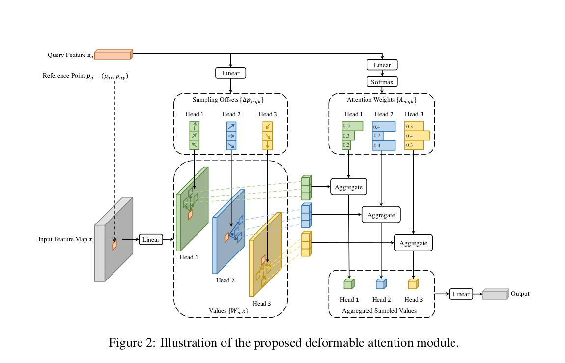

Deformable Attention


# Split the value tensor into per-level chunks based on spatial shapes
value_list = value.split([h * w for h, w in spatial_shapes_list], dim=1)
batch_size, _, num_heads, hidden_dim = value.shape

# Print the shape of each level's value tensor
for level, feature in enumerate(value_list):
    print(f"Splitted feature at level {level} --> {feature.shape}")

# Convert normalized sampling locations from [0, 1] to [-1, 1] for grid_sample
sampling_grids = 2 * sampling_location - 1
print(f"\nSampling grid shape  = {sampling_grids.shape} \n")

sampling_value_list = []

for level_id, (height, width) in enumerate(spatial_shapes_list):
    # Reshape value tensor for grid sampling:
    # (B, H*W, num_heads, C) → (B, num_heads, H*W, C) → (B*num_heads, C, H, W)
    value_l = (
        value_list[level_id]
        .flatten(2)               # (B, H*W, num_heads * C)
        .transpose(1, 2)          # (B, num_heads * C, H*W)
        .reshape(batch_size * num_heads, hidden_dim, height, width)
    )
    print(f"Value at level {level_id} {value_l.shape}")

    # Reshape sampling grid:
    # (B, num_queries, num_heads, num_levels, num_points, 2)
    # → (B, num_heads, num_queries, num_points, 2)
    # → (B*num_heads, num_queries, num_points, 2)
    sampling_grid_l = sampling_grids[:, :, :, level_id].transpose(1, 2).flatten(0, 1)

    # Sample values using bilinear interpolation
    sampling_value_l = nn.functional.grid_sample(
        value_l,
        sampling_grid_l,
        mode="bilinear",
        padding_mode="zeros",
        align_corners=False,
    )

    sampling_value_list.append(sampling_value_l)

Splitted feature at level 0 --> torch.Size([4, 17956, 8, 32])
Splitted feature at level 1 --> torch.Size([4, 4489, 8, 32])
Splitted feature at level 2 --> torch.Size([4, 1156, 8, 32])
Splitted feature at level 3 --> torch.Size([4, 289, 8, 32])

Sampling grid shape  = torch.Size([4, 23890, 8, 4, 4, 2]) 

Value at level 0 torch.Size([32, 32, 134, 134])
Value at level 1 torch.Size([32, 32, 67, 67])
Value at level 2 torch.Size([32, 32, 34, 34])
Value at level 3 torch.Size([32, 32, 17, 17])

for f in sampling_value_list:
    print(f.shape)

torch.Size([32, 32, 23890, 4])
torch.Size([32, 32, 23890, 4])
torch.Size([32, 32, 23890, 4])
torch.Size([32, 32, 23890, 4])

final_key_matrix = torch.stack(sampling_value_list, dim=-2)
print(f"Stacked value matrix shape before flattening = {final_key_matrix.shape}")
final_key_matrix = final_key_matrix.flatten(-2)
print(f"Stacked value matrix shape after flattening = {final_key_matrix.shape}")

Stacked value matrix shape before flattening = torch.Size([32, 32, 23890, 4, 4])
Stacked value matrix shape after flattening = torch.Size([32, 32, 23890, 16])

attention_weights = attention_weights.transpose(1, 2).reshape(
            batch_size * num_heads, 1, num_queries, num_levels * n_points
        )
attention_weights.shape

torch.Size([32, 1, 23890, 16])

output = final_key_matrix*attention_weights
output.shape

torch.Size([32, 32, 23890, 16])

output = output.sum(-1)
output.shape

torch.Size([32, 32, 23890])

output = output.view(batch_size,num_heads*hidden_dim,num_queries).transpose(1,2)
output = output_projection_layer(output)
output.shape

torch.Size([4, 23890, 256])

# Feed forward layers 
hidden_states = nn.functional.dropout(hidden_states,p=0.1)
hidden_states = inputs_embeds + hidden_states # residual
hidden_states = layer_norm1(hidden_states)

residual = hidden_states
hidden_states = nn.ReLU()(fc1(hidden_states))
hidden_states = nn.functional.dropout(hidden_states,p=0.1)
hidden_states = fc2(hidden_states)
hidden_states  = nn.functional.dropout(hidden_states,p=0.1)

hidden_states = residual+hidden_states
hidden_states = layer_norm2(hidden_states)

hidden_states.shape

torch.Size([4, 23890, 256])

The above hidden state acts as the input to the next decoder layer, here i am showing only one decoder layer and in the paper they used 8, the output of the final decoder layer will be passed as input to the decoder for cross attention.

Transformer Decoder

The decoder follows the same overall design as DETR but with key modifications for efficiency:

1. Learnable Object Queries

The decoder starts with a fixed set of learnable queries (300 in the paper) and learnable positional embeddings.
These queries represent potential objects and are refined through multiple decoder layers.

2. Self-Attention

The first step is self-attention among the 300 queries, this is similar to the DETR paper.

3. Cross-Attention with Deformable Attention

The second step is cross-attention between the decoder queries and the encoder’s multi-scale feature maps.
Instead of standard dense attention (which was the case in DETR), Deformable DETR uses multi-scale deformable attention, similar to the encoder:
- Each query predicts a reference point in normalized coordinates.
- Two lightweight networks predict:
  - Sampling offsets for each attention head and feature level.
  - Attention weights for the sampled points.
- For each query:
  - K = 4 sampling points per level, across L = 4 levels, giving 16 points total.
  - Features at these fractional locations are extracted using bilinear interpolation.
  - The weighted sum of these sampled features forms the cross-attention output.

How this helps!!

This design avoids attending to all pixels, reducing complexity from quadratic to linear in spatial size.
It also aligns attention with predicted object locations, improving convergence and detection accuracy.

📺 Watch the Explanation in Youtube

Deformable Decoder

encoder_output = hidden_states.clone()
num_query = 300
embedding_dim = encoder_output.shape[-1]
num_levels
# Learnable query and positional embeddings
position_embeddings = nn.Parameter(torch.randn(num_query, embedding_dim)) #(num_query,embedding_dim)
position_embeddings = position_embeddings[None].expand(batch_size,-1,-1) # (batch_size,num_query,embedding_dim)
input_query = nn.Parameter(torch.randn(num_query, embedding_dim)) #(num_query,embedding_dim)
input_query = input_query[None].expand(batch_size,-1,-1) # (batch_size,num_query,embedding_dim) 

fc1 = nn.Linear(embdedding_dim, 512)
fc2 = nn.Linear(512, embdedding_dim)

layer_norm1 = nn.LayerNorm(embdedding_dim)
layer_norm2 = nn.LayerNorm(embdedding_dim)
layer_norm3 = nn.LayerNorm(embedding_dim)

# Linear layer to generate reference points from positional embeddings
decoder_reference_point_layer = nn.Linear(embedding_dim, 2)

# Generate normalized reference points in [0, 1] range
reference_points = decoder_reference_point_layer(position_embeddings).sigmoid()  # shape: (num_query, 2)
print(f"Encode Reference points shape {reference_points.shape}")

Encode Reference points shape torch.Size([4, 300, 2])

reference_points_input = reference_points[:,:,None,:].expand(batch_size,num_query,num_levels,2)
reference_points_input.shape

torch.Size([4, 300, 4, 2])

# Initially here we will have the normal self attention.
residual = input_query
multihead_attn = nn.MultiheadAttention(embedding_dim, num_heads)
self_attn_output, _ = multihead_attn(input_query+position_embeddings, input_query+position_embeddings, input_query)
hidden_state_after_self_attention = self_attn_output + residual # residual connection. 
hidden_state_after_self_attention = layer_norm1(hidden_state_after_self_attention)
second_residual = hidden_state_after_self_attention 
print(f"Hidden state shape input to cross attention  {self_attn_output.shape}")

Hidden state shape input to cross attention  torch.Size([4, 300, 256])

position_embeddings.shape,hidden_state_after_self_attention.shape,encoder_output.shape

(torch.Size([4, 300, 256]),
 torch.Size([4, 300, 256]),
 torch.Size([4, 23890, 256]))

## DEFORMABLE MULTI SCALE ATTENTION.
num_heads = 8
num_levels  = 4
n_points  = 4
embdedding_dim = hidden_state_after_self_attention.shape[-1]
batch_size, num_queries, _ = hidden_state_after_self_attention.shape

# learnable parameters in the layer
sampling_offsets_layer = nn.Linear(embdedding_dim, num_heads * num_levels * n_points *2)
attention_weights_layer = nn.Linear(embdedding_dim,num_heads * num_levels * n_points)
value_projection_layer  = nn.Linear(embdedding_dim,embdedding_dim)
output_projection_layer = nn.Linear(embdedding_dim,embdedding_dim)

#initially we add the poistional_embedding to the input_embeds
hidden_states = hidden_state_after_self_attention + position_embeddings
value = value_projection_layer(encoder_output)
_,encoder_sequence_length,_ = value.shape
value = value.view(batch_size,encoder_sequence_length, num_heads,embdedding_dim//num_heads)
print(f"Value shape = {value.shape}")

# note for the below sampling offset and attention weights we are using the hidden state which have positional embedding information in it.
sampling_offsets = sampling_offsets_layer(hidden_states)
sampling_offsets = sampling_offsets.view(batch_size,num_queries,num_heads,num_levels,n_points,2) 
# sampling_offsets are predicted in a normalized, unitless space (not tied to any particular feature map size).
# Each feature map (level) can have a different spatial resolution (height, width).
# To convert the offsets into actual positions on each feature map, they must be scaled relative to that map's size.

offset_normalizer = torch.tensor(spatial_shapes_list)
offset_normalizer = offset_normalizer[None,None,None,:,None,:]
sampling_offsets = sampling_offsets/offset_normalizer
print(f"Offset Normalizer {offset_normalizer.shape}")

attention_weights = attention_weights_layer(hidden_states)
attention_weights = attention_weights.view(batch_size,num_queries,num_heads,num_levels*n_points)
# note here the softmax is along a row of size 16 ,intuitively this means there 4 points from 4 feature levels
attention_weights = torch.nn.functional.softmax(attention_weights, -1).view(batch_size,num_queries,num_heads,num_levels,n_points) 
print(f"Sampling offset shape = {sampling_offsets.shape}")
print(f"Attention weights shape = {attention_weights.shape} \n")


# Now we have to modify the refrence points with these sampling points, what this means is that for each of the reference points ,
# we need to look into 4 more points across 8 different heads
# so initially we had for each query 1 points account each feature dimension making it total 4 and 
# now when we add this sampling offsets it makes 4 more across 8 differenet heads
reference_points_input = reference_points_input[:,:,None,:,None,:]
print(f"Reference points with unsqueezed dimension for head and levels = {reference_points_input.shape}")
sampling_location = reference_points_input + sampling_offsets
print(f"Final sampling locations = {sampling_location.shape}")

Value shape = torch.Size([4, 23890, 8, 32])
Offset Normalizer torch.Size([1, 1, 1, 4, 1, 2])
Sampling offset shape = torch.Size([4, 300, 8, 4, 4, 2])
Attention weights shape = torch.Size([4, 300, 8, 4, 4]) 

Reference points with unsqueezed dimension for head and levels = torch.Size([4, 300, 1, 4, 1, 2])
Final sampling locations = torch.Size([4, 300, 8, 4, 4, 2])

Deformable Attention

# Split the value tensor into per-level chunks based on spatial shapes
value_list = value.split([h * w for h, w in spatial_shapes_list], dim=1)
batch_size, _, num_heads, hidden_dim = value.shape

# Print the shape of each level's value tensor
for level, feature in enumerate(value_list):
    print(f"Splitted feature at level {level} --> {feature.shape}")

# Convert normalized sampling locations from [0, 1] to [-1, 1] for grid_sample
sampling_grids = 2 * sampling_location - 1
print(f"\nSampling grid shape  = {sampling_grids.shape} \n")

sampling_value_list = []

for level_id, (height, width) in enumerate(spatial_shapes_list):
    # Reshape value tensor for grid sampling:
    # (B, H*W, num_heads, C) → (B, num_heads, H*W, C) → (B*num_heads, C, H, W)
    value_l = (
        value_list[level_id]
        .flatten(2)               # (B, H*W, num_heads * C)
        .transpose(1, 2)          # (B, num_heads * C, H*W)
        .reshape(batch_size * num_heads, hidden_dim, height, width)
    )
    print(f"Value at level {level_id} {value_l.shape}")

    # Reshape sampling grid:
    # (B, num_queries, num_heads, num_levels, num_points, 2)
    # → (B, num_heads, num_queries, num_points, 2)
    # → (B*num_heads, num_queries, num_points, 2)
    sampling_grid_l = sampling_grids[:, :, :, level_id].transpose(1, 2).flatten(0, 1)

    # Sample values using bilinear interpolation
    sampling_value_l = nn.functional.grid_sample(
        value_l,
        sampling_grid_l,
        mode="bilinear",
        padding_mode="zeros",
        align_corners=False,
    )

    sampling_value_list.append(sampling_value_l)

Splitted feature at level 0 --> torch.Size([4, 17956, 8, 32])
Splitted feature at level 1 --> torch.Size([4, 4489, 8, 32])
Splitted feature at level 2 --> torch.Size([4, 1156, 8, 32])
Splitted feature at level 3 --> torch.Size([4, 289, 8, 32])

Sampling grid shape  = torch.Size([4, 300, 8, 4, 4, 2]) 

Value at level 0 torch.Size([32, 32, 134, 134])
Value at level 1 torch.Size([32, 32, 67, 67])
Value at level 2 torch.Size([32, 32, 34, 34])
Value at level 3 torch.Size([32, 32, 17, 17])

for i,f in enumerate(sampling_value_list):
    print(f"Sampling points from each layer {i} {f.shape}")

Sampling points from each layer 0 torch.Size([32, 32, 300, 4])
Sampling points from each layer 1 torch.Size([32, 32, 300, 4])
Sampling points from each layer 2 torch.Size([32, 32, 300, 4])
Sampling points from each layer 3 torch.Size([32, 32, 300, 4])

final_key_matrix = torch.stack(sampling_value_list, dim=-2)
print(f"Stacked value matrix shape before flattening = {final_key_matrix.shape}")
final_key_matrix = final_key_matrix.flatten(-2)
print(f"Stacked value matrix shape after flattening = {final_key_matrix.shape}")

Stacked value matrix shape before flattening = torch.Size([32, 32, 300, 4, 4])
Stacked value matrix shape after flattening = torch.Size([32, 32, 300, 16])

attention_weights = attention_weights.transpose(1, 2).reshape(
            batch_size * num_heads, 1, num_queries, num_levels * n_points
        )
attention_weights.shape

torch.Size([32, 1, 300, 16])

output = final_key_matrix*attention_weights
print(f"Output after attention {output.shape}")
output = output.sum(dim=-1)
print(f"Final output after summation {output.shape}")
output = output.view(batch_size,num_heads*hidden_dim,num_queries).transpose(1,2)
print(f" Output reshaped --> {output.shape}")
output = output_projection_layer(output)

Output after attention torch.Size([32, 32, 300, 16])
Final output after summation torch.Size([32, 32, 300])
 Output reshaped --> torch.Size([4, 300, 256])

output.shape

torch.Size([4, 300, 256])

hidden_states = nn.functional.dropout(output,p=0.1)
hidden_states = second_residual + hidden_states
hidden_states = layer_norm2(hidden_states)

# Fully connected
residual = hidden_states
hidden_states = nn.ReLU()(fc1(hidden_states))
hidden_states = fc2(hidden_states)
hidden_states = hidden_states + residual
hidden_states = layer_norm3(hidden_states)

encoder_output = hidden_states.clone()
encoder_output.shape

torch.Size([4, 300, 256])

Final Box and class prediction

After the decoder produces object query embeddings, two heads operate in parallel:

Classification Head
A linear layer maps each query embedding to class logits (e.g., 10 classes). The authors uses Sigmoid + Focal Loss for multi-label classification
Box Regression Head
A small feed-forward network predicts four values: offsets for ((x, y, w, h)) in logit space (unconstrained).
- The query’s reference point (normalized in ([0,1])) is converted to logit space using inverse sigmoid.
- Offsets are added to this reference point for the center coordinates.
- Finally, a sigmoid maps the result back to normalized coordinates ([0,1]^4), giving the final bounding box.

This design stabilizes training because the network learns relative offsets in an unconstrained space rather than directly regressing normalized coordinates, which accelerates convergence and improves accuracy.

# This is needed because  model predicts an offset in unconstrained space 
# By applying inverse_sigmoid(reference_points), we map the reference points from [0, 1] to unconstrained space,
# which is  the same space as the predicted offset.
# Then bring it back to the constrained space , by appling sigmoid, this making learning faster.

reference_points_with_inverse_sigmoid = torch.special.logit(reference_points)

# say we have 10 classes
num_class = 10 
class_pred = nn.Linear(embdedding_dim,num_class)
box_head  = nn.Sequential(
    nn.Linear(embdedding_dim, 512),
    nn.ReLU(inplace=True),
    nn.Linear(512, 4),
)

output_classes = class_pred(encoder_output)
box_pred = box_head(encoder_output)
box_pred[...,:2] += reference_points_with_inverse_sigmoid
pred_boxes = box_pred.sigmoid()
print(f"Final box head shape {output_classes.shape}")
print(f"Final pred boxes head shape {pred_boxes.shape} ")

Final box head shape torch.Size([4, 300, 10])
Final pred boxes head shape torch.Size([4, 300, 4])

# Losses are similart to DETR, only difference is Deformable detr uses focal loss for  classification and for pred boxes,
# it uses the same loss like DETR where the losses are a combination of l1 loss and Generalized IOU loss

Deformable Attention: Compute and Memory Complexity

📺 Watch the Explanation in Youtube

Deformable Decoder

The paper have a good summary of the complexity of the computation here I will show it bit in detail, specializing to the encoder and decoder settings, and show how $L$ (levels) and $K$ (points per level) enter the formulas.

Notation

$N_q$: number of queries
$N_k$: number of keys
$M$: number of heads
$C$: channel dimension
$C_v = C/M$: per-head dimension
$H \times W$: spatial size of a single feature map
$H_l \times W_l$: spatial size at level $l$
$S = \sum_{l=1}^L H_l W_l$: total token count across levels
$K$: sampled points per head per level
$L$: number of feature levels

0) Preliminaries: What Contributes to Cost?

For any attention block, there are four compute buckets:

Linear projections to form $Q, K, V$ (and the output projection): costs scale like $\mathcal{O}(N C^2)$.
Score computation (e.g., $QK^\top$ or its sparse substitute): costs scale like $\mathcal{O}(N_q N_k C_v M) = \mathcal{O}(N_q N_k C)$ for dense attention.
Softmax + weighting: typically $\mathcal{O}(N_q N_k M)$ for softmax, and $\mathcal{O}(N_q N_k C)$ for multiplying by $V$; the latter usually dominates.
Sampling / Interpolation (deformable attention only): adds a term of approximately $\mathcal{O}(N_q \cdot \text{\#samples} \cdot C)$; Appendix of the paper counts this as a constant “5” times per sample for bilinear interpolation + reduct

Memory is dominated by storing the attention weights: $\mathcal{O}(N_q N_k M)$ for dense vs. $\mathcal{O}(N_q M K)$ (single-scale) or $\mathcal{O}(N_q M L K)$ (multi-scale).

1) Standard Multi-Head Attention (Expression is directly from the paper Eq1)

\[ \text{MultiHeadAttn}(z_q, x) = \sum_{m=1}^M W_m \sum_{k \in \mathcal{K}} A_{mqk} W'_m x_k \]

Compute:

Projections:
- $Q$: $\mathcal{O}(N_q C^2)$
- $K, V$: $\mathcal{O}(N_k C^2)$
Scores ($QK^\top$): $\mathcal{O}(M \cdot N_q N_k C_v) = \mathcal{O}(N_q N_k C)$
Softmax: $\mathcal{O}(M \cdot N_q N_k)$
Weighted sum (AV): $\mathcal{O}(M \cdot N_q N_k C_v) = \mathcal{O}(N_q N_k C)$
Output projection: $\mathcal{O}(N_q C^2)$

Total (dense attention):

\[ \boxed{\mathcal{O}\big(N_q C^2 + N_k C^2 + N_q N_k C\big)} \]

Memory:

Attention weights: $\mathcal{O}(M N_q N_k)$ (dominant)
Key/value caches: $\mathcal{O}(N_k C)$

Specializations:

DETR encoder (self-attention over pixels): $N_q = N_k = S$

\[ \mathcal{O}(S^2 C) + \mathcal{O}(S C^2) \quad \text{(dominated by $S^2C$)} \]
DETR decoder cross-attention: $N_q = N$ queries, $N_k = S$ pixels

\[ \mathcal{O}(N S C) + \mathcal{O}((N+S)C^2) \]
DETR decoder self-attention (queries only):

\[ \mathcal{O}(2 N C^2 + N^2 C) \]

2) Single-Scale Deformable Attention (Expression is directly from the paper Eq2)

\[ \text{DeformAttn}(z_q, p_q, x) = \sum_{m=1}^M W_m \sum_{k=1}^K A_{mqk} W'_m x(p_q + p_{mqk}) \]

Each query attends $K$ sampled points per head around reference $p_q$. Sampling uses bilinear interpolation.

Predict offsets + weights (a single linear with $3MK$ output channels over $z_q$): $\mathcal{O}(3 N_q C M K)$
Value projection ($W'_m x$): two possible ways
- Precompute once on the whole map: $\mathcal{O}(H W C^2)$
- Or do per sampled value: $\mathcal{O}(N_q K C^2)$
Sampling + weighted sum (bilinear + reduce): approx 5 ops per sample per channel: $\mathcal{O}(5 N_q K C)$
Output projection: $\mathcal{O}(N_q C^2)$

Putting it together (App. A.1):

\[ \boxed{ \mathcal{O}\Big(N_q C^2 + \min(H W C^2, N_q K C^2) + 5 N_q K C + 3 N_q C M K\Big) } \]

For typical settings ($M=8$, $K \leq 4$, $C=256$), the paper notes $5K + 3MK \ll C$, yielding the simplification:

\[ \boxed{\mathcal{O}\big(2 N_q C^2 + \min(H W C^2, N_q K C^2)\big)} \]

Memory:

Attention weights: $\mathcal{O}(M N_q K)$
Offsets: $\mathcal{O}(M N_q K \cdot 2)$
No dense $(N_q \times N_k)$ matrix—this is the major win.

Specializations:

Encoder (single-scale, queries are pixels): $N_q = HW$
With precomputation ($W'_m x$): complexity becomes $\mathcal{O}(HW C^2)$, i.e. linear in spatial size (vs. quadratic for dense).
Decoder cross-attention (single-scale): $N_q = N$
With per-query sampled values: $\mathcal{O}(N K C^2)$ (independent of $HW$).

3) Multi-Scale Deformable Attention ( Expression is directly from the paper Eq. (3))

\[ \text{MSDeformAttn}(z_q, \hat{p}_q, \{x_l\}_{l=1}^L) = \sum_{m=1}^M W_m \sum_{l=1}^L \sum_{k=1}^K A_{mlqk} W'_m x_l(\phi_l(\hat{p}_q) + p_{mlqk}) \]

Each query samples $(L \times K)$ points total.

Compute:

Predict offsets + weights: $\mathcal{O}(3 N_q C M L K)$
Value projections (choose one):
- Precompute on all levels: $\sum_{l=1}^L \mathcal{O}(H_l W_l C^2) = \mathcal{O}(S C^2)$
- Or per sampled value: $\mathcal{O}(N_q L K C^2)$
Sampling + weighted sum: $\mathcal{O}(5 N_q L K C)$
Output projection: $\mathcal{O}(N_q C^2)$

Total (multi-scale):

\[ \boxed{ \mathcal{O}\Big(N_q C^2 + \min(S C^2, N_q L K C^2) + 5 N_q L K C + 3 N_q C M L K\Big) } \]

Under the same “small $(M, K, L)$” assumption as the paper (App. A.1):

\[ \boxed{ \mathcal{O}\big(2 N_q C^2 + \min(S C^2, N_q L K C^2)\big) } \]

Memory:

Attention weights: $\mathcal{O}(M N_q L K)$
Offsets: $\mathcal{O}(M N_q L K \cdot 2)$
Again, no dense $(N_q \times S)$ matrix.

Specializations:

Deformable DETR encoder (multi-scale, queries are pixels across all levels): $N_q = S$
Precompute values per level $\rightarrow$ \[ \boxed{\mathcal{O}(S C^2)} \quad \text{(linear in total tokens across scales)} \] This is the paper’s claim that encoder complexity becomes linear in spatial size (Section 4.1).
Deformable DETR decoder cross-attention: $N_q = N$ queries
Use per-query samples $\rightarrow$ \[ \boxed{\mathcal{O}(N L K C^2)} \quad \text{(independent of spatial resolution)} \]
Decoder self-attention: unchanged from standard: $\mathcal{O}(2 N C^2 + N^2 C)$.

4) Comparison of the above three

Block	Dense MHA (DETR)	Deformable (single-scale)	Deformable (multi-scale)
Generic	$\mathcal{O}(N_q C^2 + N_k C^2 + N_q N_k C)$	$\mathcal{O}(2 N_q C^2 + \min(HW C^2, N_q K C^2))$	$\mathcal{O}(2 N_q C^2 + \min(S C^2, N_q L K C^2))$
Encoder	$N_q = N_k = S \Rightarrow \mathcal{O}(S^2 C)$	$N_q = HW \Rightarrow \mathcal{O}(HW C^2)$	$N_q = S \Rightarrow \boxed{\mathcal{O}(S C^2)}$
Decoder cross-attn	$N_q = N, N_k = S \Rightarrow \mathcal{O}(N S C)$	$\mathcal{O}(N K C^2)$	$\boxed{\mathcal{O}(N L K C^2)}$
Decoder self-attn	$\mathcal{O}(2 N C^2 + N^2 C)$	same	same
Attention memory	$\mathcal{O}(M N_q N_k)$	$\mathcal{O}(M N_q K)$	$\mathcal{O}(M N_q L K)$

5) How Deformable Detr is Better

Encoder: dense self-attention is quadratic in spatial tokens; deformable makes it linear in the total number of tokens across scales ($S$).
Decoder cross-attention: deformable cost depends on $(L K)$ (small, fixed hyperparameters), not on image size, so it scales with the number of queries ($N$) and channel dimension ($C$), not with $H, W$.
Memory: deformable avoids the $\mathcal{O}(N_q N_k)$ attention matrix, replacing it with $\mathcal{O}(N_q L K)$ structures—crucial for speed and convergence.

Key Improvements of Deformable DETR over DETR

DETR needs 500 epochs to reach ~42 AP, while Deformable DETR achieves 43.8 AP in just 50 epochs.
Training time drops drastically: 325 GPU hours vs. 2000+ for DETR.
Inference speed: Deformable DETR runs at 19 FPS, faster than DETR-DC5 (12 FPS).
Deformable DETR converges 10× faster than DETR-DC5.

Credits

Most of the implementation closely follow the below two, so all credtits to them!!

Block	Dense MHA (DETR)	Deformable (single-scale)	Deformable (multi-scale)
Generic	\(\mathcal{O}(N_q C^2 + N_k C^2 + N_q N_k C)\)	\(\mathcal{O}(2 N_q C^2 + \min(HW C^2, N_q K C^2))\)	\(\mathcal{O}(2 N_q C^2 + \min(S C^2, N_q L K C^2))\)
Encoder	\(N_q = N_k = S \Rightarrow \mathcal{O}(S^2 C)\)	\(N_q = HW \Rightarrow \mathcal{O}(HW C^2)\)	\(N_q = S \Rightarrow \boxed{\mathcal{O}(S C^2)}\)
Decoder cross-attn	\(N_q = N, N_k = S \Rightarrow \mathcal{O}(N S C)\)	\(\mathcal{O}(N K C^2)\)	\(\boxed{\mathcal{O}(N L K C^2)}\)
Decoder self-attn	\(\mathcal{O}(2 N C^2 + N^2 C)\)	same	same
Attention memory	\(\mathcal{O}(M N_q N_k)\)	\(\mathcal{O}(M N_q K)\)	\(\mathcal{O}(M N_q L K)\)